SQL (Structured Query Language)

 

SQL

Follow me

SQL Definition:

            SQL stands for Structured Query Language. It is a language used to communicate with and manage databases. With SQL, you can perform various tasks like retrieving data, updating data, and organizing the structure of a database.

Using SQL, you are able to interact with the database by writing queries, which when executed, return any results which meet its criteria. 

Here’s an example query:-

                SELECT * FROM users;

Using this SELECT statement, the query selects all data from all columns in the user’s table. It would then return data like the below, which is typically called a results set:- 

If we were to replace the asterisk wildcard character (*) with specific column names instead, only the data from these columns would be returned from the query

                SELECT first_name, last_name FROM users; 

We can add a bit of complexity to a standard SELECT statement by adding a WHERE clause, which allows you to filter what gets returned.

SELECT * FROM products WHERE stock_count <= 10 ORDER BY stock_count ASC; 

This query would return all data from the products table with a stock_count value of less than 10 in its results set. The use of the ORDER BY keyword means the results will be ordered using the stock_count column, lowest values to highest.

Using the INSERT INTO statement, we can add new data to a table. Here’s a basic example adding a new user to the users table:-

INSERT INTO users (first_name, last_name, address, email)

VALUES (‘Tester’, ‘Jester’, ‘123 Fake Street, Sheffield, United Kingdom’, ‘test@lukeharrison.dev’);

Then if you were to rerun the query to return all data from the user’s table, the results set would look like this:

Of course, these examples demonstrate only a very small selection of what the SQL language is capable of.

SQL vs MYSQL

SQL and MySQL are related but serve different purposes. Here's an easy explanation of the difference between them:

SQL (Structured Query Language)

• What it is: SQL is a language used to interact with and manage databases. It's a set of commands used to create, retrieve, update, and delete data in a database.
• Purpose: SQL is used for querying and managing the data inside a database, regardless of which database system you're using.
• Examples of SQL commands: SELECT, INSERT, UPDATE, DELETE, CREATE, ALTER, etc.
• Scope: SQL is a standard language used by many database systems.

MySQL

• What it is: MySQL is a relational database management system (RDBMS) that uses SQL as its language for managing data. It is a software that stores and manages your data using SQL commands.
• Purpose: MySQL is the database system that you use to actually store and manage your data. It allows multiple users to interact with the database through SQL.
• Examples of MySQL use: Creating a database, managing tables, handling user access, etc.
• Scope: MySQL is a specific database product, like Oracle, SQL Server, or PostgreSQL. It uses SQL to handle the data.

Key Differences:

1. SQL is the language used for querying databases, while MySQL is a software/database system that uses SQL to perform actions.
2. SQL can be used with various database systems like MySQL, Oracle, SQL Server, etc., but MySQL specifically refers to a database software that implements SQL.
3. SQL itself is just the language, while MySQL is the tool that stores and manages the data based on SQL commands.

In short, SQL is the language for database management, and MySQL is a system that uses SQL to manage and organize data.

Download and Install of MySQL

Download and Install MySQL on your computer:

Step 1: Download MySQL

1. Go to the official MySQL website:
   Open your browser and go to https://dev.mysql.com/downloads/installer/.

2. Choose your version:
   You will see two options: MySQL Installer for Windows and MySQL Community Server. Choose the first one: MySQL Installer for Windows.

3. Download the installer:
   You will be given an option to download either the 32-bit or 64-bit version. Most modern systems use the 64-bit version, so select that if you're unsure.

4. Start the download:
   Click the “Download” button. If it asks you to log in, you can skip it by clicking on "No thanks, just start my download."

Step 2: Run the MySQL Installer

1. Locate the downloaded file:
   Once the download is complete, find the installer file (usually in your Downloads folder) and double-click it to start the installation.

2. Choose setup type:
   When you run the installer, you will be asked to choose a setup type. Select "Developer Default" for most users, as this will install MySQL along with useful tools like MySQL Workbench.

3. Download and install dependencies:
   The installer might prompt you to download additional files. Just follow the instructions, and it will download and install everything you need.

Step 3: Configure MySQL

1. Choose MySQL server version:
   After the installation of necessary components, you'll be prompted to choose the version of MySQL to install. Choose the latest version and proceed.

2. Set a root password:
   The installer will ask you to set a root password. This is the main password for accessing the MySQL server. Make sure to remember it.

3. Choose other options (optional):
   You can select additional configurations, such as enabling MySQL as a Windows service, which means MySQL will start automatically when your computer boots up. You can also choose the port (default is 3306).

4. Apply the configuration:
   After you’ve selected your options, click “Next” and then “Execute” to apply the changes and set up MySQL.

Step 4: Complete the Installation

1. Finish the installation:
   Once MySQL is successfully installed, you’ll see a screen that confirms everything is set up correctly. Click Finish to close the installer.

Step 5: Test the MySQL Installation

1. Open MySQL Workbench:
   If you selected the Developer Default setup, MySQL Workbench should have been installed. Open it to connect to your MySQL server.

2. Log in to MySQL:

   • Open MySQL Workbench.
   • Under MySQL Connections, click on the Local instance MySQL (it may say “3306”).
   • When prompted, enter the root password you set earlier.
   • You should now be connected to your MySQL server.

3. Test by running a simple query:
   In MySQL Workbench, type and execute this command to check if everything is working:

   SELECT VERSION();

   If you get a version number, it means MySQL is installed and running properly!

Optional: Access MySQL via Command Line

1. Open Command Prompt:
   You can also access MySQL from the command line. Press Win + R, type cmd, and press Enter.

2. Access MySQL:
   Type the following command to log into MySQL:

   mysql -u root -p

   Then enter your root password when prompted. You should now be inside the MySQL command line interface.

Introduction to SQL Keywords

In SQL, the keywords are the reserved words that are used to perform various operations in the database. There are many keywords in SQL, and as SQL is case insensitive, it does not matter if we use, for example, SELECT or select.

List of SQL Keywords

The examples below explain that SQL keywords can be used for various operations.

1. CREATE

The CREATE Keyword is used to create a database, table, views, and index. We can create the table CUSTOMER as below.

CREATE TABLE CUSTOMER (CUST_ID INT PRIMARY KEY, NAME VARCHAR(50), STATE VARCHAR(20));

2. PRIMARY KEY

This keyword uniquely identifies each of the records.

A Database in SQL can be created with the usage of CREATE DATABASE statement as below:

CREATE DATABASE DATABASE_NAME;

A View in SQL can be created by using CREATE VIEW as below:

CREATE VIEW VIEW_NAME AS
SELECT COLUMN1, COLUMN2, COLUMN3...
FROM TABLE_NAME WHERE [CONDITION];

3. INSERT

The INSERT Keyword is used to insert the rows of data into a table. We can insert the rows below to the already created CUSTOMER table using the queries below.

INSERT INTO CUSTOMER VALUES (121,'Rajesh','Maharashtra');
INSERT INTO CUSTOMER VALUES(256,'Leela','Punjab');
INSERT INTO CUSTOMER VALUES(908,'Priya','Jharkhand');
INSERT INTO CUSTOMER VALUES(787,'Rohit','UP');

The above statements will insert the rows to the table “CUSTOMER”. We can see the result by using a simple SELECT statement below

SELECT * FROM CUSTOMER;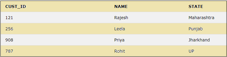

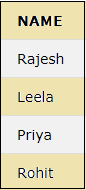
4. SELECT

This keyword is used to select the data from the database or table. The ‘*’ is used in the select statement to select all the columns in a table.

SELECT NAME FROM CUSTOMER; 

The result of the above query will display the column NAME from the CUSTOMER table below.

5. FROM

The keyword indicates the table from which the data is selected or deleted.

6. ALTER

The Keyword ALTER is used to modify the columns in tables. The ALTER COLUMN statement modifies the data type of a column, and the ALTER TABLE modifies the columns by adding or deleting them.

We can modify the columns of the CUSTOMER table as below by adding a new column, “AGE”.

ALTER TABLE CUSTOMER ADD AGE INT;
SELECT * FROM CUSTOMER;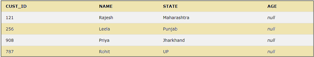

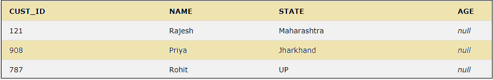
This query above will add the new column “AGE” with values for all the rows as null. Also, the above statement uses another SQL keyword ‘ADD’.

7. ADD

This is used to add a column to the existing table.

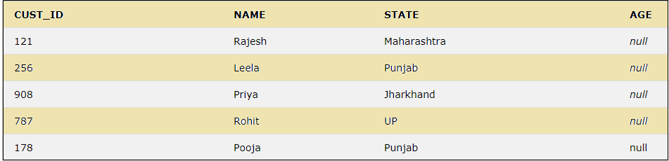
8. DISTINCT

The keyword DISTINCT is used to select distinct values. We can use SELECT DISTINCT to select only the distinct values from a table.

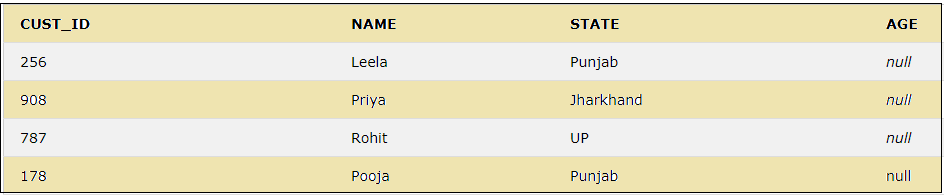
Let us add a duplicate value for the state Punjab as below:

INSERT INTO CUSTOMER VALUES(178, 'Pooja', 'Punjab','null');

The customer table now has the below rows:

Now we can see the distinct values for the column STATE by using the below query:

SELECT DISTINCT(STATE) FROM CUSTOMER;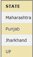

9. UPDATE

This keyword is used in an SQL statement to update the existing rows in a table.

UPDATE CUSTOMER SET STATE ='Rajasthan' WHERE CUST_ID= 121;
SELECT * FROM CUSTOMER;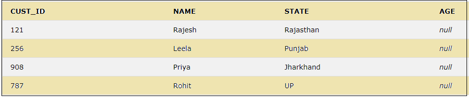

The CUST_ID with value 121 is updated with a new state Rajasthan.

10. SET

This Keyword is used to specify the column or values to be updated.

11. DELETE

This is used to delete the existing rows from a table.

DELETE FROM CUSTOMER WHERE NAME='Rajesh';

The above query will display the below as the row with Name as Rajesh is deleted from the result set.

While using the DELETE keyword, if we do not use the WHERE clause, all the records will be deleted from the table.

DELETE FROM CUSTOMER;

The above query will delete all the records of the CUSTOMER table.

12. TRUNCATE

This is used to delete the data in a table, but it does not delete the structure of the table.

TRUNCATE TABLE CUSTOMER;

The above query only deletes the data, but the structure of the table remains. So there is no need to re-create the table.

13. AS

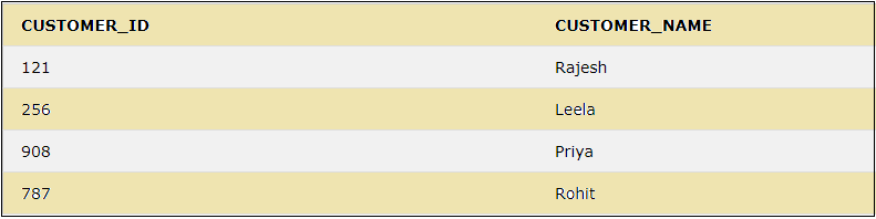
The Keyword AS is used as an alias to rename the column or table.

SELECT CUST_ID AS CUSTOMER_ID, NAME AS CUSTOMER_NAME FROM CUSTOMER;

The above statement will create the alias for the columns CUST_ID and NAME as below:

14. ORDER BY

This is used to sort the result in descending or ascending order. This sorts the result by default in ascending order.

15. ASC

 This keyword is used for sorting the data returned by the SQL query in ascending order.

SELECT * FROM CUSTOMER ORDER BY NAME ASC;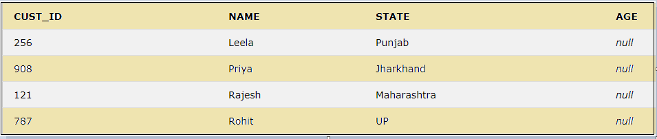

The above query will select all the columns from the CUSTOMER table and sorts the data by the NAME column in ascending order.

16. DESC

This keyword is to sort the result set in descending order.

SELECT * FROM CUSTOMER ORDER BY CUST_ID DESC;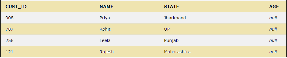

The above query will sort all the selected fields of the table in the descending order of CUST_ID.

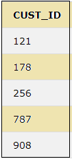
17. BETWEEN

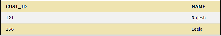
This keyword is used to select values within a given range. The below query uses the BETWEEN keyword to select the CUST_ID and NAME within a given range of values for the CUST_ID.

SELECT CUST_ID, NAME FROM CUSTOMER WHERE CUST_ID BETWEEN 100 AND 500;

The above query will give the below result

18. WHERE

This keyword is used to filter the result set so that only the values satisfying the condition are included.

SELECT * FROM CUSTOMER WHERE STATE ='Punjab';

The above query selects all the values from the table for which the state is Punjab.

19. AND

This keyword is used along with the WHERE clause to select the rows for which both conditions are true.

SELECT * FROM CUSTOMER WHERE STATE ='Punjab' AND CUST_ID= 256;

The above query will give the result as mentioned below.

But if one of the conditions is not satisfied, then the query will not return any result, as stated in the below query.

SELECT * FROM CUSTOMER WHERE STATE ='Punjab' AND CUST_ID= 121;

20. OR

This is used with the WHERE clause to include the rows in the result set in case of either condition is true.

The below SQL statement will select the fields from the CUSTOMER table if the state is Punjab or UP.

SELECT * FROM CUSTOMER WHERE STATE='Punjab' OR STATE='UP';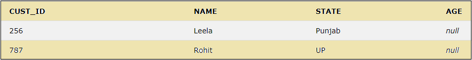

In the case of the OR keyword, we can see from the above result that if any of the given conditions are true, that gets included in the result set.

21. NOT

The keyword NOT uses a WHERE clause to include the rows in the result set where a condition is not true.

We can use the NOT keyword in the below query to not include the rows from the state Punjab as below.

SELECT * FROM CUSTOMER WHERE NOT STATE = 'Punjab';

The query will return the rows with the other states, excluding Punjab in the result set as below:

22. LIMIT

This keyword retrieves the records from the table to limit them based on the limit value.

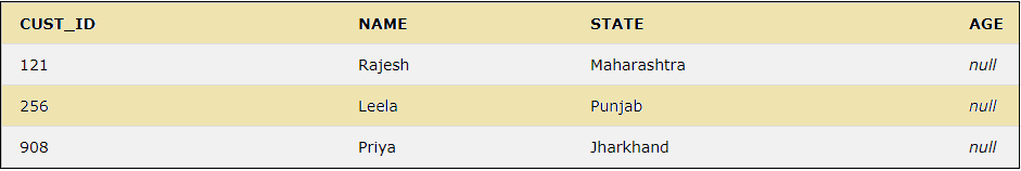
SELECT * FROM CUSTOMER LIMIT 3;

The above query will select the records from the table CUSTOMER, but it will display only the 3 rows of data from the table as below

23. IS NULL

The keyword IS NULL is used to check for NULL values.

The below query will show all the records for which the AGE column has NULL values.

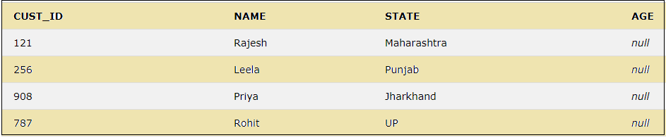
SELECT * FROM CUSTOMER WHERE AGE IS NULL;

IS NOT NULL

This is used to search the NOT NULL values.

SELECT * FROM CUSTOMER WHERE STATE IS NOT NULL;

As the column STATE has no null values, the above query will show the below result.

24. DROP

The DROP keyword can be used to delete a database, table, view, column, index, etc.

25. DROP COLUMN

We can delete an existing column in a table using a DROP COLUMN and an ALTER statement. Let us delete the column AGE by using the below query.

ALTER TABLE CUSTOMER DROP COLUMN AGE;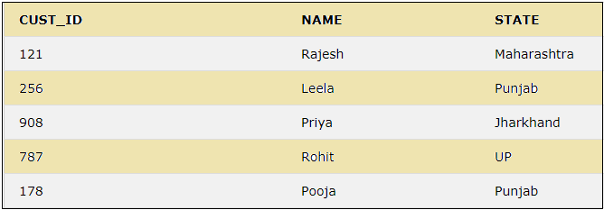

We can see that in the above result, the AGE column is dropped.

26. DROP DATABASE

A database in SQL can be deleted by using the DROP DATABASE statement.

DROP DATABASE DATABASE_NAME;

27. DROP TABLE

A table in SQL can be deleted by using a DROP TABLE statement.

DROP TABLE TABLE_NAME;

We can delete the table CUSTOMER by using the DROP TABLE keyword as below.

But we must be careful while using the DROP TABLE as it will remove the table definition, all the data, indexes, etc.

28. GROUP BY

This is used along with the aggregate functions like COUNT, MAX, MIN, AVG, SUM, etc., and groups the result set. The below query will group the CUST_ID according to the various states.

SELECT COUNT(CUST_ID),STATE FROM CUSTOMER GROUP BY STATE;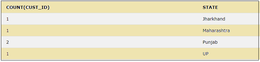

The result shows the count of different CUST_ID grouped by states.

29. HAVING

This keyword is used with aggregate functions and GROUP BY instead of the WHERE clause to filter the values of a result set.

SELECT COUNT(CUST_ID),STATE FROM CUSTOMER GROUP BY STATE HAVING COUNT(CUST_ID)>=2;

The above query will filter the result set by displaying only those values which satisfy the condition given in the HAVING clause.

The above result set shows the values for which the count of the customer ids is more than 2.

30. IN

The IN keyword is used within a WHERE clause to specify more than 1 value, or we can say that it can be used instead of the usage of multiple OR keyword in a query.

The query below will select the records for the states Maharashtra, Punjab, and UP by using the IN keyword.

SELECT * FROM CUSTOMER WHERE STATE IN ('Maharashtra','Punjab','UP');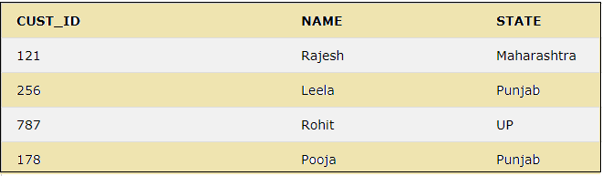

The above result shows the usage of IN keyword, which selects the records only for the states specified within the IN clause.

31. JOIN

The keyword JOIN combines the rows between two or more tables with related columns among the tables. The JOIN can be INNER, LEFT, RIGHT, OUTER JOIN, etc.

Lets us take another table, ‘CUST_ORDER’, as an example.

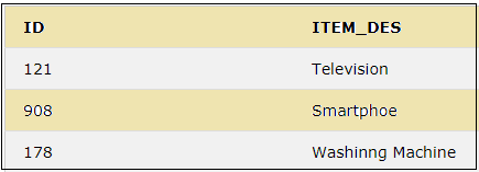
We can perform an inner join of the CUSTOMER and CUST_ORDER tables as below.

SELECT CUSTOMER.NAME, CUSTOMER.STATE, CUST_ORDER.ITEM_DES
FROM CUSTOMER INNER JOIN CUST_ORDER
ON CUSTOMER.CUST_ID =CUST_ORDER.ID;

The above query will join the two tables CUSTOMER and CUST_ORDER on the columns CUST_ID and ID and display only the values which are present in both tables.

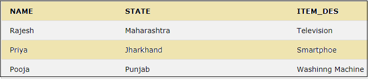
This result shows the matching records for cust_id 121,908 and 178, which are common in both tables. But the other cust_ids are excluded as they are not present in the CUST_ORDER table. Similarly, the other JOINs can be performed.

32. UNION

The UNION keyword combines the distinct values of two or more select statements.

SELECT CUST_ID FROM CUSTOMER UNION SELECT ID FROM CUST_ORDER;

The above query will show the below result.

33. UNION ALL

This keyword combines two or more select statements but allows duplicate values.

SELECT CUST_ID FROM CUSTOMER UNION ALL SELECT ID FROM CUST_ORDER;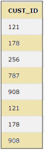

The above result shows that UNION ALL allows duplicate values which would not be present in the case of UNION.

34. EXISTS

The keyword EXISTS checks if a certain record exists in a sub-query.

SELECT NAME FROM CUSTOMER WHERE EXISTS (SELECT ITEM_DES FROM CUST_ORDER WHERE CUST_ID = ID);

The above query will return true as the sub-query returns the below values.

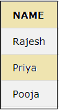
35. LIKE

This keyword is used to search along with a WHERE clause for a particular pattern. Wildcard % is used to search for a pattern.

In the below query, let us search for a pattern ‘ya’ which occurs in the column ‘NAME’.

SELECT NAME FROM CUSTOMER WHERE NAME LIKE '%ya';

36. CASE

This keyword is used to display different outputs according to different conditions.

SELECT CUST_ID, NAME,
CASE WHEN STATE = 'Punjab' THEN "State is Punjab"
ELSE "State is NOT Punjab"
END AS Output
FROM CUSTOMER;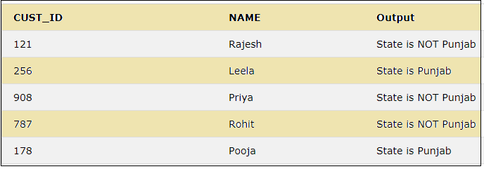

A few other keywords are DEFAULT, used to provide a default value for a column, UNIQUE, used to ensure all the values in a column are unique; etc.

Comment

In SQL, comments are used to add explanatory notes to the code. They are ignored by the SQL engine and do not affect the execution of queries. You can add comments to your SQL code for better readability and understanding, especially when working with complex queries.

There are two types of comments in SQL:

1. Single-line comments: Use -- to comment a single line of code.
2. Multi-line comments: Use /* to start and */ to end a comment block.

Example Single-Line Comment

-- Select all:
SELECT * FROM Customers;

In the above example, the comment -- This is a single-line comment is a note for developers. It doesn't affect the query execution.

Example Multi-Line Comment

/*Select all the columns
of all the records
in the Customers table:*/
SELECT * FROM Customers;

In the above example, everything between /* and */ is treated as a comment, allowing you to write multi-line explanations.

Brief Explanation:

• Single-line comments are useful for short explanations or to comment out a single line of code temporarily.
• Multi-line comments are helpful when you need to explain a large block of code or write more detailed descriptions.

Both types of comments are commonly used for:

• Clarifying the logic of queries.
• Providing context for the code.
• Temporarily disabling code during testing or debugging.

String Data Types

In SQL, string data types are used to store text values. These data types allow you to store strings of varying lengths and characteristics. Below is a list of common string data types in SQL, along with explanations and examples.

1. CHAR (n)

• Description: The CHAR data type is used to store fixed-length strings. If the string is shorter than the specified length n, it will be padded with spaces to the right to match the defined length.
• Use Case: Ideal for storing values with a consistent length (e.g., country codes, state abbreviations)

In this case, the value 'USA' would be stored as 'USA ' (padded with two spaces to reach 5 characters).

2. VARCHAR (n)

• Description: The VARCHAR (variable-length character) data type is used to store strings with a variable length, up to the maximum specified length n. Unlike CHAR, VARCHAR does not add padding to shorter strings.
• Use Case: Suitable for storing strings where the length can vary, like names, email addresses, and descriptions.

In this case, 'example@example.com' would be stored exactly as is, without any padding.

3. TEXT

• Description: The TEXT data type is used to store large strings of text. It is similar to VARCHAR, but can store much larger amounts of data (in some databases, it can store up to 65,535 characters or more).
• Use Case: Ideal for long text entries such as articles, blog posts, or detailed descriptions.

The TEXT field can hold much larger content than VARCHAR.

4. NCHAR (n)

• Description: The NCHAR data type is similar to CHAR, but it stores Unicode characters (i.e., multi-byte characters) for international or special characters.
• Use Case: Useful for storing characters in different languages or non-latin scripts.

Here, the NCHAR data type would store the Japanese characters, ensuring correct encoding.

5. NVARCHAR (n)

• Description: The NVARCHAR data type is similar to VARCHAR, but it stores Unicode characters, allowing for a wider range of characters from different languages.
• Use Case: Ideal for storing variable-length Unicode strings like names, addresses, or descriptions in various languages.

The NVARCHAR type ensures that the Chinese characters are correctly stored.

6. LONGTEXT

• Description: Similar to TEXT, but LONGTEXT can store much larger amounts of data (in some databases, up to 4GB of text).
• Use Case: Suitable for very large pieces of text, such as large documents or detailed logs.

Example of Creating a Table with Different String Data Types:

In this table:

• username is a variable-length string up to 50 characters.
• bio is a large block of text.
• country_code is a fixed-length 3-character string for storing country codes.
• full_name is a variable-length Unicode string that can support different languages.

Number Data Types

In SQL, number data types are used to store numerical values, either integers or decimals. Different database systems may have variations in the types available, but the general concept remains the same. Below is a list of common number data types in SQL, along with explanations and example code.

1. INT (INTEGER)

• Description: The INT data type is used to store whole numbers (integers) without a fractional part. The size of INT may vary depending on the database system, but typically it can store values from -2^31 to 2^31-1.
• Use Case: Used for counting, IDs, or any other whole number data.

In this example, user_id is an integer that can store whole numbers.

2. SMALLINT

• Description: The SMALLINT data type is similar to INT, but it is designed to store smaller integer values. The range of SMALLINT typically goes from -32,768 to 32,767.
• Use Case: Suitable for storing smaller values, such as age or number of items in a small inventory.

Here, quantity is a smaller integer that doesn't need the full range of INT.

3. TINYINT

• Description: The TINYINT data type is used for very small integers. Its range is typically from -128 to 127 (or 0 to 255 for unsigned).
• Use Case: Used when storing small values like flags, statuses, or small counts.

In this example, status is a tiny integer (e.g., 0 or 1) representing a simple on/off or true/false state.

4. BIGINT

• Description: The BIGINT data type is used to store large integers. The range typically goes from -2^63 to 2^63-1.
• Use Case: Used for storing large numeric values, such as large counts, timestamps, or unique IDs.

The large_number field can store very large integers, useful for high-traffic applications or systems generating large IDs.

5. DECIMAL(p, s) or NUMERIC(p, s)

• Description: Both DECIMAL and NUMERIC are used for storing exact fixed-point numbers with a specified precision p (total number of digits) and scale s (number of digits after the decimal point).
• Use Case: Suitable for monetary values, percentages, or any other precise numerical calculation where rounding is not acceptable.

In this case, price is a decimal number with up to 10 digits, of which 2 are after the decimal point. This ensures that values like money are stored with precision.

6. FLOAT

• Description: The FLOAT data type is used to store approximate numeric values with floating-point precision. The storage size can vary, but FLOAT typically provides 7 digits of precision (for 4-byte float). Precision and scale can vary depending on the database system.
• Use Case: Used for scientific or engineering calculations that require approximate values.

In this example, measurement stores a floating-point number, suitable for values that don't require exact precision.

7. DOUBLE (or DOUBLE PRECISION)

• Description: The DOUBLE data type is used to store approximate numeric values, similar to FLOAT, but with double precision. DOUBLE typically offers 15–16 digits of precision.
• Use Case: Suitable for calculations that require greater precision than FLOAT.

In this case, distance is stored with double precision, which allows for higher accuracy than FLOAT.

8. REAL

• Description: The REAL data type is a synonym for FLOAT in some databases, typically representing a single-precision floating-point number with 4-byte storage.
• Use Case: Used for approximate values, similar to FLOAT, but with less precision.

The temperature field stores a floating-point value.

Example of Creating a Table with Numeric Data Types:

In this table:

• transaction_id stores the ID of the transaction.
• amount stores the monetary amount with precision.
• tax_rate stores a floating-point number representing the tax rate.
• balance stores a very large integer value for account balance or similar large quantities.

Date and Time Data Types

Operators in SQL

1. Arithmetic Operators

• + : Addition
• - : Subtraction
• * : Multiplication
• / : Division
• % : Modulo (remainder after division)

2. Comparison Operators

• = : Equal to
• <> or != : Not equal to
• > : Greater than
• < : Less than
• >= : Greater than or equal to
• <= : Less than or equal to
• BETWEEN : Range check (within a range)
• IN : Checks if a value matches any value in a list
• LIKE : Pattern matching (typically used with wildcards)
• IS NULL : Checks if a value is NULL

3. Logical Operators

• AND : Combines multiple conditions; true if both conditions are true
• OR : Combines multiple conditions; true if at least one condition is true
• NOT : Negates a condition; true if the condition is false

4. String Operators

• CONCAT : Combines two or more strings into one
• || : Concatenates two strings (used in some SQL variants like PostgreSQL)
• LIKE : Pattern matching for strings (e.g., using wildcards like % and _)
• ILIKE : Case-insensitive version of LIKE (used in PostgreSQL)

5. Set Operators

• UNION : Combines the result sets of two queries (removes duplicates)
• UNION ALL : Combines the result sets of two queries (including duplicates)
• INTERSECT : Returns the common records from two queries
• EXCEPT : Returns the records from the first query that are not in the second query

6. Bitwise Operators (Supported in some databases)

• & : Bitwise AND
• | : Bitwise OR
• ^ : Bitwise XOR
• ~ : Bitwise NOT
• << : Bitwise shift left
• >> : Bitwise shift right

7. Null-related Operators

• IS NULL : Checks if a value is NULL
• IS NOT NULL : Checks if a value is not NULL
• COALESCE : Returns the first non-NULL value in a list of arguments
• NULLIF : Returns NULL if two values are equal, otherwise returns the first value

8. Existence Operators

• EXISTS : Checks if a subquery returns any results
• NOT EXISTS : Checks if a subquery returns no results

9. Other Operators

• ANY : Compares a value to any value in a list or subquery
• ALL : Compares a value to all values in a list or subquery
• SOME : Similar to ANY; checks if a condition is true for at least one value in a subquery

Functions in SQL

1. Aggregate Functions

• COUNT(): Returns the number of rows that match a specified condition.
• SUM(): Calculates the total sum of a numeric column.
• AVG(): Calculates the average of a numeric column.
• MIN(): Returns the smallest value in a specified column.
• MAX(): Returns the largest value in a specified column.
• GROUP_CONCAT(): Concatenates values from multiple rows into a single string (typically used in MySQL).
• ARRAY_AGG(): Aggregates values from multiple rows into an array (used in PostgreSQL).

2. String Functions

• CONCAT(): Concatenates two or more strings into a single string.
• LENGTH(): Returns the number of characters in a string.
• SUBSTRING(): Extracts a portion of a string.
• UPPER(): Converts a string to uppercase.
• LOWER(): Converts a string to lowercase.
• TRIM(): Removes leading and trailing spaces from a string.
• REPLACE(): Replaces occurrences of a substring with another string.
• INSTR(): Returns the position of the first occurrence of a substring in a string.
• POSITION(): Finds the position of a substring in a string (standard SQL).
• LEFT(): Returns a specified number of characters from the left of a string.
• RIGHT(): Returns a specified number of characters from the right of a string.

3. Mathematical Functions

• ABS(): Returns the absolute value of a number.
• ROUND(): Rounds a numeric value to a specified number of decimal places.
• CEIL() or CEILING(): Returns the smallest integer greater than or equal to a given number.
• FLOOR(): Returns the largest integer less than or equal to a given number.
• POWER(): Returns the result of a number raised to a specified power.
• SQRT(): Returns the square root of a number.
• MOD(): Returns the remainder when one number is divided by another (modulo operation).
• RAND(): Generates a random number between 0 and 1.
• PI(): Returns the value of pi.

4. Date and Time Functions

• NOW(): Returns the current date and time.
• CURRENT_DATE(): Returns the current date.
• CURRENT_TIME(): Returns the current time.
• DATE(): Extracts the date part of a datetime or timestamp.
• TIME(): Extracts the time part of a datetime or timestamp.
• YEAR(): Extracts the year part of a date.
• MONTH(): Extracts the month part of a date.
• DAY(): Extracts the day part of a date.
• DATE_ADD(): Adds a specified time interval to a date.
• DATE_SUB(): Subtracts a specified time interval from a date.
• DATEDIFF(): Returns the difference in days between two dates.
• TIMESTAMPDIFF(): Returns the difference between two timestamps in a specific unit (e.g., years, months, days).
• EXTRACT(): Extracts a specific part (e.g., year, month, day) from a date or timestamp.

5. Conditional Functions

• CASE: Performs conditional logic in SQL (similar to if-else statements).
• COALESCE(): Returns the first non-NULL value in a list of expressions.
• NULLIF(): Returns NULL if two values are equal, otherwise returns the first value.
• IFNULL() or ISNULL(): Returns a specified value if the expression is NULL, otherwise returns the expression.

6. Conversion Functions

• CAST(): Converts a value from one data type to another.
• CONVERT(): Converts a value from one data type to another (alternative to CAST, specific to some databases like SQL Server).
• TO_CHAR(): Converts a number or date to a string.
• TO_DATE(): Converts a string to a date (used in some databases like Oracle).
• TO_NUMBER(): Converts a string to a number (used in some databases like Oracle).

7. Window Functions

• ROW_NUMBER(): Assigns a unique sequential integer to rows within a result set.
• RANK(): Assigns a rank to each row within a partition of a result set.
• DENSE_RANK(): Similar to RANK(), but without gaps in ranking for ties.
• NTILE(): Divides rows into a specified number of groups.
• LEAD(): Provides access to the value of a column in the following row in the result set.
• LAG(): Provides access to the value of a column in the previous row in the result set.
• FIRST_VALUE(): Returns the first value in an ordered partition of a result set.
• LAST_VALUE(): Returns the last value in an ordered partition of a result set.
• NTH_VALUE(): Returns the nth value in an ordered partition of a result set.

8. JSON Functions (for databases that support JSON)

• JSON_OBJECT(): Creates a JSON object from key-value pairs.
• JSON_ARRAY(): Creates a JSON array from a list of values.
• JSON_EXTRACT(): Extracts a value from a JSON object.
• JSON_SET(): Modifies a JSON object by setting a value for a specified key.
• JSON_ARRAYAGG(): Aggregates values into a JSON array.
• JSON_AGG(): Aggregates results into a JSON object or array.

9. User-Defined Functions (UDFs)

• These are custom functions created by users within a specific database to extend the functionality of SQL. UDFs are specific to the database platform.

10. Other Functions

• VERSION(): Returns the version of the database system.
• USER(): Returns the current database user.
• DATABASE(): Returns the name of the current database.
• SESSION_USER(): Returns the session user.
• LAST_INSERT_ID(): Returns the most recent auto-generated ID from an insert operation (MySQL, SQL

Wildcard Characters

Keys in SQL

1. Primary Key

A primary key uniquely identifies each record in a table. It cannot have NULL values and must be unique.

CREATE TABLE Employees (
    EmployeeID INT PRIMARY KEY,
    FirstName VARCHAR(50),
    LastName VARCHAR(50),
    Age INT
);

In this example, EmployeeID is the primary key that uniquely identifies each employee.

2. Foreign Key

A foreign key is used to establish a relationship between two tables. It points to a primary key in another table.

CREATE TABLE Departments (
    DepartmentID INT PRIMARY KEY,
    DepartmentName VARCHAR(50)
);

CREATE TABLE Employees (
    EmployeeID INT PRIMARY KEY,
    FirstName VARCHAR(50),
    LastName VARCHAR(50),
    DepartmentID INT,
    FOREIGN KEY (DepartmentID) REFERENCES Departments(DepartmentID)
);

In this example, DepartmentID in the Employees table is a foreign key that references the DepartmentID in the Departments table.

3. Unique Key

A unique key ensures that all values in a column (or combination of columns) are unique, but unlike the primary key, it allows for NULL values.

CREATE TABLE Employees (
    EmployeeID INT PRIMARY KEY,
    Email VARCHAR(100) UNIQUE,
    FirstName VARCHAR(50),
    LastName VARCHAR(50)
);

In this example, Email is a unique key, ensuring that each employee's email is unique across the table.

4. Composite Key

A composite key is a combination of two or more columns used to uniquely identify a record. It’s necessary when no single column is unique enough by itself.

CREATE TABLE CourseRegistrations (
    StudentID INT,
    CourseID INT,
    RegistrationDate DATE,
    PRIMARY KEY (StudentID, CourseID)
);

In this example, the combination of StudentID and CourseID serves as the composite primary key to uniquely identify each registration.

5. Candidate Key

A candidate key is any column or set of columns that could be used as a primary key. Only one of the candidate keys will be selected as the primary key.

CREATE TABLE Employees (
    EmployeeID INT PRIMARY KEY,
    SSN VARCHAR(11) UNIQUE,  -- Candidate Key
    FirstName VARCHAR(50),
    LastName VARCHAR(50)
);

Here, both EmployeeID and SSN are candidate keys, but EmployeeID is chosen as the primary key.

6. Alternate Key

An alternate key is a candidate key that was not chosen as the primary key.

CREATE TABLE Employees (
    EmployeeID INT PRIMARY KEY,
    SSN VARCHAR(11) UNIQUE,  -- Alternate Key
    FirstName VARCHAR(50),
    LastName VARCHAR(50)
);

In this example, SSN is an alternate key because it could also uniquely identify employees, but EmployeeID is the primary key.

7. Super Key

A super key is a set of one or more columns that can uniquely identify a record. It may contain unnecessary columns.

CREATE TABLE Employees (
    EmployeeID INT,
    SSN VARCHAR(11),
    FirstName VARCHAR(50),
    LastName VARCHAR(50),
    PRIMARY KEY (EmployeeID)
);

In this example, (EmployeeID, SSN) can also be a super key because the combination uniquely identifies records. However, it's unnecessary to use both columns as a key when EmployeeID alone is sufficient.

8. Natural Key

A natural key uses naturally occurring data to uniquely identify records.

CREATE TABLE Students (
    NationalID VARCHAR(20) PRIMARY KEY,
    FirstName VARCHAR(50),
    LastName VARCHAR(50)
);

In this case, the NationalID is a natural key, as it’s a real-world identifier that can uniquely identify students.

9. Surrogate Key

A surrogate key is an artificially created key, usually a simple auto-incrementing integer, that has no business meaning.

CREATE TABLE Students (
    StudentID INT AUTO_INCREMENT PRIMARY KEY,
    FirstName VARCHAR(50),
    LastName VARCHAR(50)
);

In this example, StudentID is a surrogate key because it is auto-generated and does not have any real-world business meaning.

10. Clustering Key

A clustering key is used to determine the physical order of rows in the table (common in clustered indexes). Some databases like MySQL or SQL Server automatically create a clustering key when a primary key is defined.

CREATE TABLE Orders (
    OrderID INT PRIMARY KEY,
    OrderDate DATE,
    CustomerID INT,
    TotalAmount DECIMAL(10, 2)
);

In this example, OrderID is the clustering key because the rows in the table will be stored in the order of OrderID (since it’s the primary key).

11. Unique Constraint

A unique constraint ensures that all values in a specified column or combination of columns are unique.

CREATE TABLE Employees (
    EmployeeID INT PRIMARY KEY,
    Email VARCHAR(100),
    PhoneNumber VARCHAR(15),
    CONSTRAINT unique_phone UNIQUE (PhoneNumber)
);

Indexes

In SQL, indexes are used to speed up the retrieval of rows from a database table. They are like a "shortcut" for querying the data. Below are the different types of indexes in SQL, along with simple example code to explain each.

1. Simple Index

A simple index is created on a single column to speed up the search for values in that column.

CREATE INDEX idx_employee_lastname ON Employees (LastName);

• Explanation: This index is created on the LastName column of the Employees table. It speeds up queries that filter or sort by LastName.

2. Unique Index

A unique index ensures that the values in the indexed column(s) are unique. It is automatically created for primary keys and unique constraints.

CREATE UNIQUE INDEX idx_unique_email ON Employees (Email);

• Explanation: This unique index ensures that each value in the Email column is unique. If you try to insert a duplicate email, the database will reject the insertion.

3. Composite Index

A composite index (also called a multi-column index) is created on multiple columns to optimize queries that use more than one column in the WHERE clause.

CREATE INDEX idx_employee_name_age ON Employees (FirstName, Age);

• Explanation: This index is created on the FirstName and Age columns of the Employees table. It helps speed up queries that filter by both FirstName and Age.

4. Full-Text Index

A full-text index is used for performing text searches in large text fields (like TEXT or VARCHAR columns). It allows you to search for words within the text.

CREATE FULLTEXT INDEX idx_fulltext_description ON Products (Description);

• Explanation: This full-text index is created on the Description column of the Products table. It allows you to perform full-text searches (e.g., searching for specific words within product descriptions).

5. Clustered Index

A clustered index determines the physical order of rows in a table. Each table can have only one clustered index, and it is typically created on the primary key by default.

CREATE CLUSTERED INDEX idx_clustered_employee_id ON Employees (EmployeeID);

• Explanation: This index is created on the EmployeeID column of the Employees table, and it will determine the physical order of the rows. By default, the primary key is often the clustered index.

6. Non-Clustered Index

A non-clustered index creates a separate structure from the data table and contains pointers to the actual data. You can have multiple non-clustered indexes on a table.

CREATE NONCLUSTERED INDEX idx_nonclustered_lastname ON Employees (LastName);

• Explanation: This creates a non-clustered index on the LastName column of the Employees table. It improves the speed of queries that search or filter by LastName, but does not affect the physical order of rows in the table.

7. Spatial Index

A spatial index is used for spatial data types (like geographical data) and helps optimize spatial queries.

CREATE SPATIAL INDEX idx_spatial_location ON Locations (Coordinates);

• Explanation: This index is used on the Coordinates column of the Locations table, which stores geographical data. It speeds up spatial queries like finding locations within a certain area.

8. Bitmap Index

A bitmap index is used for columns with a low cardinality (few distinct values). It's often used in decision support databases.

CREATE BITMAP INDEX idx_bitmap_gender ON Employees (Gender);

• Explanation: This index is created on the Gender column of the Employees table. It's efficient when the column has only a few distinct values (like M or F for gender).

9. Partial Index

A partial index is created only on a subset of the data, typically based on a condition in the WHERE clause.

CREATE INDEX idx_active_employees ON Employees (LastName)
WHERE Status = 'Active';

• Explanation: This index is created only on the rows where Status is 'Active'. It can help optimize queries that filter by active employees.

Joins in SQL

In SQL, joins are used to combine rows from two or more tables based on a related column between them. Here is a breakdown of the different types of joins in SQL with simple examples of code:

1. INNER JOIN

The INNER JOIN returns rows when there is a match in both tables. If there is no match, no rows are returned.

SELECT Employees.EmployeeID, Employees.FirstName, Departments.DepartmentName
FROM Employees
INNER JOIN Departments
ON Employees.DepartmentID = Departments.DepartmentID;

• Explanation: This query returns all employees along with their department names, but only for employees who have a matching department in the Departments table.

2. LEFT JOIN (or LEFT OUTER JOIN)

The LEFT JOIN returns all rows from the left table (the first table), and the matching rows from the right table (the second table). If there is no match, NULL values are returned for columns from the right table.

SELECT Employees.EmployeeID, Employees.FirstName, Departments.DepartmentName
FROM Employees
LEFT JOIN Departments
ON Employees.DepartmentID = Departments.DepartmentID;

• Explanation: This query returns all employees, including those who do not belong to any department. For employees without a department, NULL is returned in the DepartmentName column.

3. RIGHT JOIN (or RIGHT OUTER JOIN)

The RIGHT JOIN returns all rows from the right table (the second table), and the matching rows from the left table (the first table). If there is no match, NULL values are returned for columns from the left table.

SELECT Employees.EmployeeID, Employees.FirstName, Departments.DepartmentName
FROM Employees
RIGHT JOIN Departments
ON Employees.DepartmentID = Departments.DepartmentID;

• Explanation: This query returns all departments, even those that do not have any employees. For departments without employees, NULL is returned in the EmployeeID and FirstName columns.

4. FULL JOIN (or FULL OUTER JOIN)

The FULL JOIN returns all rows when there is a match in one of the tables. If there is no match, NULL values are returned for columns from the table that does not have a match.

SELECT Employees.EmployeeID, Employees.FirstName, Departments.DepartmentName
FROM Employees
FULL OUTER JOIN Departments
ON Employees.DepartmentID = Departments.DepartmentID;

• Explanation: This query returns all employees and all departments. If an employee is not assigned to a department, the DepartmentName will be NULL. If a department does not have any employees, the EmployeeID and FirstName will be NULL.

5. CROSS JOIN

The CROSS JOIN returns the Cartesian product of two tables. This means it will combine every row of the first table with every row of the second table. Be cautious with CROSS JOIN as it can result in a large number of rows.

SELECT Employees.EmployeeID, Departments.DepartmentName
FROM Employees
CROSS JOIN Departments;

• Explanation: This query returns every combination of employee and department, resulting in a Cartesian product of the two tables. If there are 3 employees and 4 departments, the result will be 12 rows (3 * 4).

6. SELF JOIN

A SELF JOIN is a join where a table is joined with itself. This is useful when you need to compare rows within the same table.

SELECT A.EmployeeID, A.FirstName AS EmployeeName, B.EmployeeID, B.FirstName AS ManagerName
FROM Employees A
INNER JOIN Employees B
ON A.ManagerID = B.EmployeeID;

• Explanation: This query finds the relationship between employees and their managers. It joins the Employees table with itself where A.ManagerID matches B.EmployeeID. A represents the employee, and B represents the manager.

Views in SQL

In SQL, a view is a virtual table that provides a way to look at data in one or more tables. It does not store data itself, but rather stores a query that retrieves data when the view is accessed. Views are commonly used for simplifying complex queries, securing data, and presenting a simplified interface to users.

Key Points About Views:

• Virtual Table: A view is like a window to the underlying table(s). It shows data from one or more tables, but it does not store the data itself.
• Read-Only or Updatable: Views can be read-only or updatable depending on how they are defined. A view can be updatable if it directly represents a single table and does not have aggregation or complex operations.
• Simplification: Views simplify complex queries by encapsulating them as a virtual table. Users can interact with the view without needing to know the underlying complexity of the data.
• Security: Views can be used to restrict access to sensitive data by exposing only specific columns or rows to the users.

Types of Views:

1. Simple View: A simple view is created based on a single table or a straightforward query.
2. Complex View: A complex view is created using multiple tables, joins, and other SQL operations like aggregation or grouping.

Creating Views in SQL:

1. Creating a View

You can create a view using the CREATE VIEW statement.

CREATE VIEW EmployeeDetails AS
SELECT EmployeeID, FirstName, LastName, DepartmentID
FROM Employees;

• Explanation: This view, EmployeeDetails, presents a simplified view of the Employees table showing only the EmployeeID, FirstName, LastName, and DepartmentID.

2. Using a View

Once a view is created, you can query it just like a regular table.

SELECT * FROM EmployeeDetails;

• Explanation: This query selects all columns from the EmployeeDetails view, which will return data from the underlying Employees table.

3. Updating Data Through a View

If the view is updatable (i.e., it does not involve any aggregation, grouping, or joins), you can modify the data via the view.

UPDATE EmployeeDetails
SET LastName = 'Smith'
WHERE EmployeeID = 1;

• Explanation: This query updates the LastName of the employee with EmployeeID = 1 in the EmployeeDetails view. The data is updated in the underlying Employees table.

4. Dropping a View

To remove a view from the database, use the DROP VIEW statement.

DROP VIEW EmployeeDetails;

• Explanation: This removes the EmployeeDetails view from the database. Note that the underlying data in the Employees table remains unaffected.

5. Creating a View with Joins (Complex View)

You can create views based on multiple tables by using SQL joins.

CREATE VIEW DepartmentEmployeeDetails AS
SELECT e.EmployeeID, e.FirstName, e.LastName, d.DepartmentName
FROM Employees e
JOIN Departments d
ON e.DepartmentID = d.DepartmentID;

• Explanation: This view, DepartmentEmployeeDetails, joins the Employees table with the Departments table and returns employee details along with their department name.

Advantages of Using Views:

• Simplification: You can simplify complex SQL queries by storing the query logic inside the view. Users can then query the view without needing to understand the underlying complexity.
• Security: Views can provide a level of abstraction, hiding sensitive or unnecessary data from users. You can control which columns or rows users can access.
• Consistency: Views allow you to create consistent data representations, which helps standardize reporting and data retrieval across applications.

Example of Using Views:

Suppose you have two tables, Employees and Departments, and you want to create a view that shows employee names along with their department name.

1. Employees Table:

   CREATE TABLE Employees (
       EmployeeID INT PRIMARY KEY,
       FirstName VARCHAR(50),
       LastName VARCHAR(50),
       DepartmentID INT
   );
   

2. Departments Table:

   CREATE TABLE Departments (
       DepartmentID INT PRIMARY KEY,
       DepartmentName VARCHAR(50)
   );
   

3. View for Employee and Department Info:

   CREATE VIEW EmployeeDepartmentInfo AS
   SELECT e.EmployeeID, e.FirstName, e.LastName, d.DepartmentName
   FROM Employees e
   JOIN Departments d
   ON e.DepartmentID = d.DepartmentID;
   

4. Query the View:

   SELECT * FROM EmployeeDepartmentInfo;
   

• Output:

  EmployeeID	FirstName	LastName	DepartmentName
  1	John	Doe	HR
  2	Jane	Smith	IT
  3	Emily	Brown	Finance

Conclusion

SQL is the foundation of data manipulation, empowering users to efficiently retrieve, manage, and analyze vast amounts of information. Its structured approach simplifies complex operations, ensuring data integrity and accessibility across platforms.